This is a writeup on the background and development of a 3-sphere visualizer, which is available here with code on GitHub.

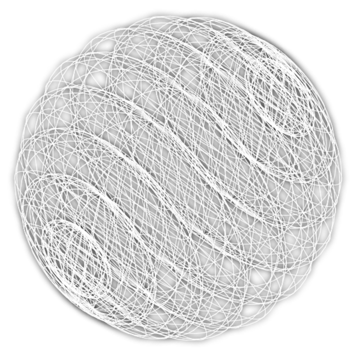
I came across this amazing image once while researching quaternions:

"2D-projection of 3D-projection of Hypersphere of 4D-space" by Eugene Antipov, CC-By-SA-2.5, 2.0, and 1.0, from 3-sphere

The picture was on the Wikipedia page "3-sphere" with caption "Direct projection of 3-sphere into 3D space and covered with surface grid, showing structure as stack of 3D spheres (2-spheres)".

I really wanted to recreate it - partly to understand it, and partly to get a higher-resolution version of the image. The original seems be a bit compressed, or maybe just lacks anti-aliasing. Either way, I think it would look stunning in greater detail.

What is the 3-sphere?

According to that Wikipedia page, the 3-sphere is the "higher-dimensional analogue of a sphere". A (regular) sphere is the boundary of a 3D ball, where a ball is a solid 3D shape. If the ball is a solid, like a marble, its surface is a sphere. One dimension higher, the 3-sphere is the surface of a solid 4D ball.

This is a complicated image to keep in one's head.

Another definition of the 3-sphere is that it is the set of points in 4D Euclidian space that are all lie at the same distance from a certain point. The lower-dimensional analogy here is how all the the 3D points on a regular sphere of radius r$r$ lie at a distance r$r$ from the sphere's center.

What is that picture?

Judging by the image title and its Wikipedia caption, I think what is going on in the picture is

1. A bunch of lines are drawn on a 3-sphere. These lines are like latitude and longitude lines on a sphere, but there is also... a third kind of line
2. Some 4D rotation might be applied
3. The lines drawn on the 3-sphere, represented by a series of line segments with 4D start and end points, are projected into 3D space by a projection matrix, yielding a bunch of line segments with 3D start and end points
4. Some 3D rotation might be applied to these points
5. The 3D line segments are projected into 2D space by applying another projection matrix to all the 3D line segment points, yielding a set of line segments with 2D start and end points.
6. The 2D line segments are drawn to the screen.

Steps 4, 5, and 6 are easy to visualize: just imagine lines of latitude and longitude drawn on a regular sphere:

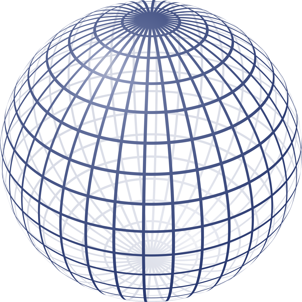
From Wikimedia Commons

The image here looks "3D", but really it's just a two-dimensional image: all the 3D lines that cover the sphere in real life have been squashed down onto a piece of paper, so to speak.

Hypermeridians

The 3-sphere Wikipedia page helpfully mentions the name of that third type of latitude/longitude line I mentioned early: if the first two types of lines are parallels (constant "latitude") and meridians (constant "longitude"), then the third type of line is the hypermeridians.

Drawing latitude and longitude lines (parallels and meridians) on a regular sphere is much easier when you work in spherical coordinates: a line of latitude is formed choosing a latitude, and then varying the longitude to draw a line that wraps around ther sphere.

To make the picture at the top of this post, we'll just need to do the same thing but in hyperspherical coordinates, as described in the same Wikipedia page.

Here is a possible mapping for hyperspherical coordinates (\psi, \theta, \phi)$(\psi, \theta, \phi)$ on a 3-sphere of radius r$r$ to 4D Cartesian coordinates (x_0, x_1, x_2, x_3)$(x_0, x_1, x_2, x_3)$:

\begin{aligned}
x_0 &= r \cos \psi \\
x_1 &= r \sin \psi \cos \theta \\
x_2 &= r \sin \psi \sin \theta \cos \phi \\
x_3 &= r \sin \psi \sin \theta \sin \phi \\
\end{aligned}

where \psi$\psi$ and \theta$\theta$ range from 0$0$ to \pi$\pi$ and \phi$\phi$ ranges from 0$0$ to 2\pi$2\pi$.

Notice that if you set \psi=\pi/2$\psi=\pi/2$, you get

\begin{aligned}
x_0 &= 0 \\
x_1 &= r \cos \theta \\
x_2 &= r \sin \theta \cos \phi \\
x_3 &= r \sin \theta \sin \phi \\
\end{aligned}

which are the equations for the parallels and meridians of a sphere in coordinates (x_1, x_2, x_3)$(x_1, x_2, x_3)$ if we call \theta$\theta$ the latitude and \phi$\phi$ the longitude!

Parallels will be constant \psi$\psi$ and \theta$\theta$, and 0 \leq \phi \lt 2\pi$0 \leq \phi \lt 2\pi$.

Meridians will be constant \psi$\psi$ and \phi$\phi$, and 0 \leq \theta \lt \pi$0 \leq \theta \lt \pi$. ^[1]

So hypermeridians will be constant \theta$\theta$ and \phi$\phi$, 0 \leq \psi \lt \pi$0 \leq \psi \lt \pi$.

Code

I chose JavaScript and HTML to do the computation and visualization for this project primarily for ease of sharing and interaction on the web.

The coded ended up being not too complicated: all I need to do is generate a set of parallels, meridians, and hypermeridians (each encoded as an array of 4D points defining a path), apply a 4D rotation to the points, and then project them down into 2D points (effectively just choosing to keep two of the four coordinates.)

Here is the first close-ish image I was able to produce:

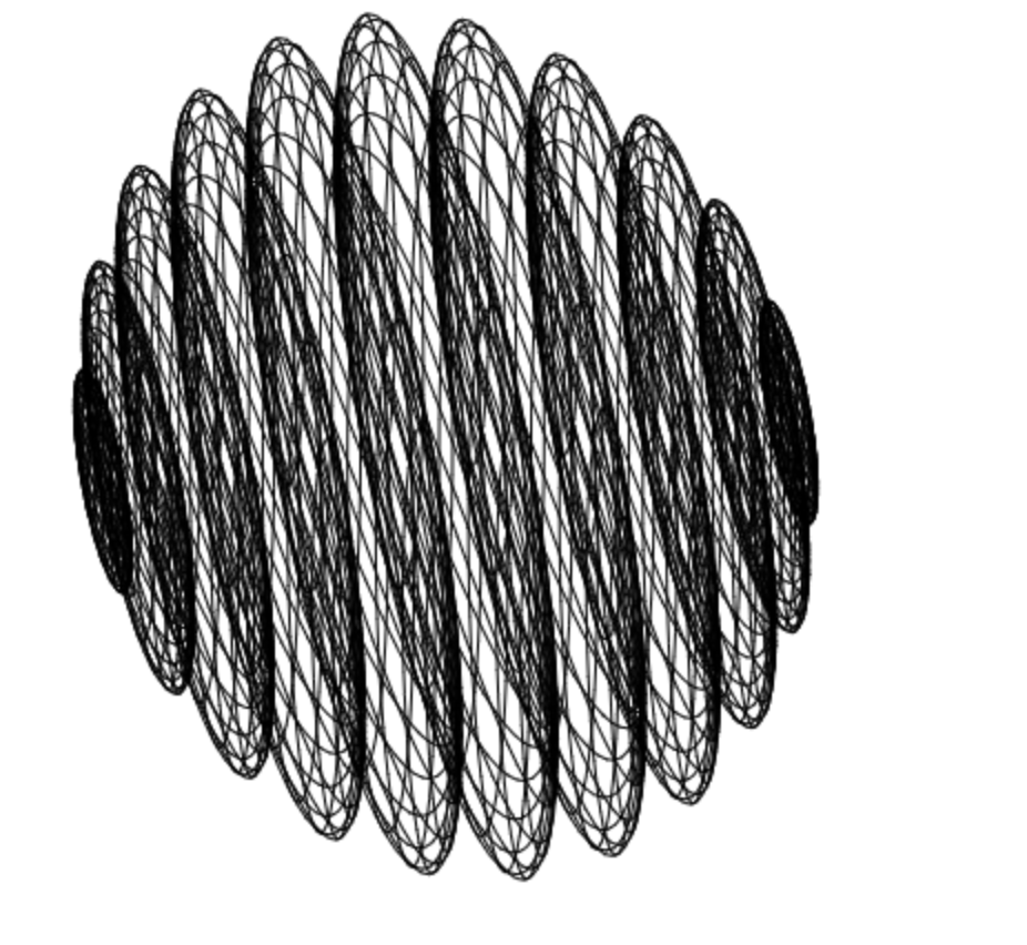
from this commit

This was really really exciting to see! It looks a bit stretched because it "rotation matrix" I apply to all the 4D points is not actually a real rotation matrix - it's just a matrix I arrived at by making small deviations from the 4D identity matrix.

Tangentially, it turns out rotations in four dimensions are not at all trivial. You might think there's just one more angle to rotation around, since in 3D there are three distinct rotations (roll, pitch, and yaw for example), but in 4D there aren't four angles that define a rotation, but six!^[2]. The Wikipedia page on 4D rotations is a cool read if you're interested. In particular, I was reading the section "Generating 4D Rotation Matrices" in an effort to add a real 4D rotation matrix to my code. It is a complicated process, but doable if you're able to find eigenvalues of a general 4D matrix, which the JavaScript math package I'm using is not. However, I realized there is a much easier way accomplish what I wanted to do.

The desired image is the the 2D "shadow" of a set of 4D lines on the 3-sphere. My original plan was to rotate all the points, and then create a 2D image by projecting all the points onto just two axes, like the x$x$ & y$y$ axes for example - effective just ignoring the 3rd and 4th components of each 4D point and drawing them on a 2D image.

However, I found it was easier to adjust the plane of projection rather than to rotate all the points. For this, I only need two 4D unit vectors, with the one constraint that they are orthogonal.^[3] Then, to draw a 4D point r$r$ in the 2D image from the , I make a 2x4 projection matrix from those vectors and multiply it with r$r$ to get the position (u,v)$(u,v)$ of the point in the projected 2D space.

\begin{bmatrix}u\\v\end{bmatrix} = \begin{bmatrix}p_w&&p_x&&p_y&&p_z\\q_w&&q_x&&q_y&&q_z\end{bmatrix} \begin{bmatrix}r_w\\r_x\\r_y\\r_z\end{bmatrix}

Whereas my original approach was similar to rotating the 3-sphere and looking at it with a camera in a fixed position, this new approach is akin to keeping the 3-sphere stationary and change the angle from which camera views it.

To make my visualization interactive, I came up with a way to apply small changes to either p$p$ or q$q$ while keeping them orthogonal. The process is to:

1. Add a small (+/- 0.1) value to one component of either p$p$ or q$q$
2. Normalize p$p$ or q$q$ to ensure it is a unit 4-vector
3. Apply the Graham-Schmidt procedure to the other vector (q$q$ or p$p$) to get an orthogonal vector that still lies in a direction close to the original.

With this "nudge and orthonormalize" process, generating different views of the 3-sphere is pretty easy. An orientation I found that gets pretty close to the original image is:

p = [0.64790, 0.12582, -0.70325, -0.26423]
q = [-0.51569, -0.61322, -0.42755, -0.41857]

p = [0.64790, 0.12582, -0.70325, -0.26423]
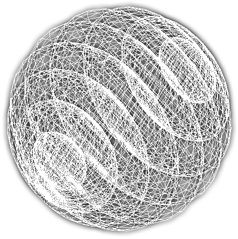
q = [-0.51569, -0.61322, -0.42755, -0.41857]

After adding enabling the HTML5 canvas property shadowBlur and drawing lines in white, I got a picture I'm very happy with:

You can play around with my 3-sphere visualization here.